LEANN Vector Index: How UC Berkeley Shrank a 201 GB RAG Index to 6 GB
LEANN, from UC Berkeley's Sky Computing Lab, keeps a pruned graph and recomputes embeddings only on the search path, shrinking a 60M-chunk RAG index from 201 GB to 6 GB. We explain how it works, check the math and test the idea with FAISS.

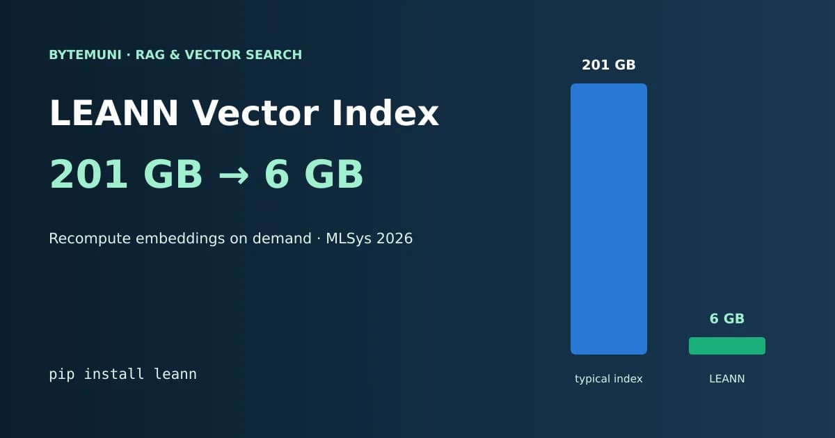
The LEANN vector index is an open-source project from UC Berkeley's Sky Computing Lab that shrinks retrieval-augmented generation (RAG) indexes by more than 95%. Instead of storing an embedding for every chunk of text, it keeps a small, pruned search graph and recomputes embeddings only for the handful of chunks each query actually visits. In the team's benchmark, a 60-million-chunk Wikipedia index drops from 201 GB to 6 GB, and the paper behind it was reported as the Best Research Paper at MLSys 2026.
That's a big deal if you've ever tried to run semantic search on your own machine. A normal vector index is often bigger than the documents it indexes. LEANN makes the index small enough for a laptop. The catch is speed: searches take seconds instead of milliseconds.
I read the paper, checked the storage math myself and ran a small FAISS experiment to test the core idea LEANN is built on. Here's what it does, how it works, where the numbers come from, when it's worth using and when it isn't.
LEANN at a glance
| Item | Detail |
|---|---|
| What it is | A low-storage approximate nearest neighbor (ANN) vector index, built on FAISS |
| Who built it | UC Berkeley Sky Computing Lab (authors include Yichuan Wang, Ion Stoica, Matei Zaharia and Joseph E. Gonzalez) |
| Core idea | Store a pruned graph and tiny compressed codes; recompute full embeddings only on the search path |
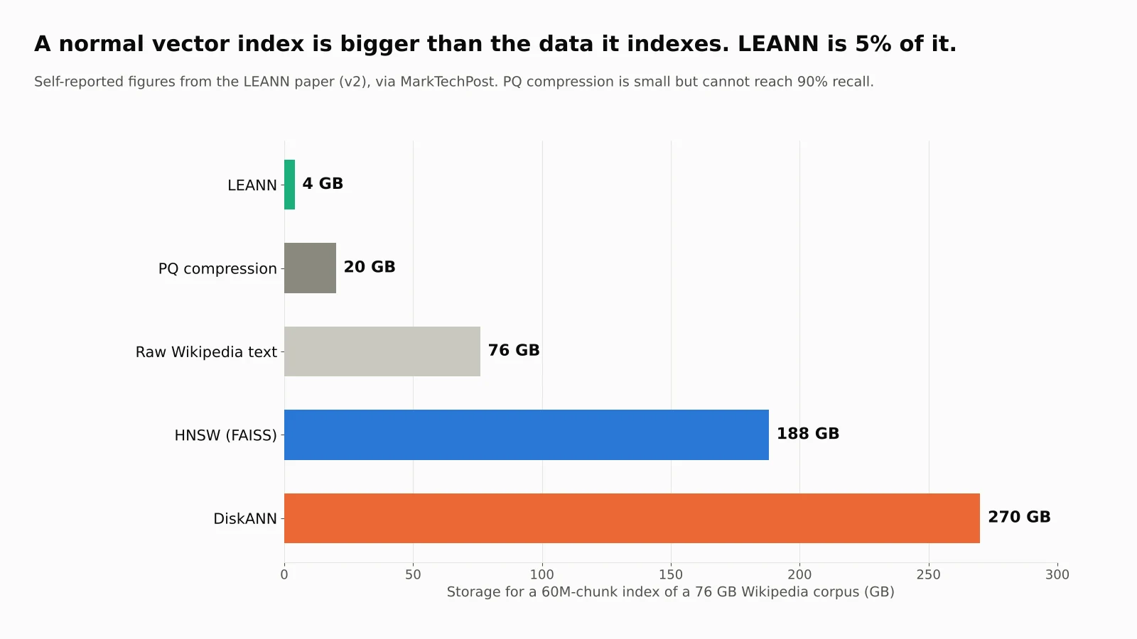
| Headline result | 60M chunks: 201 GB → 6 GB (repo benchmark); 188 GB → 4 GB for HNSW vs LEANN in the paper |
| Accuracy | Matches HNSW downstream accuracy at 90% recall (25.5% on NQ for both, self-reported) |
| Trade-off | Retrieval takes about 2.5 seconds on NQ, versus 0.05 seconds for HNSW |
| License | MIT |
| Install | uv pip install leann (or pip install leann) |
| Paper | arXiv 2506.08276 |
Why vector indexes are so big
To search text by meaning, a RAG system splits documents into chunks, turns each chunk into an embedding (a long list of numbers) and stores those embeddings in a vector index. When a question comes in, the system embeds the question and finds the chunks whose embeddings are closest.
The problem is size. The LEANN paper notes that vector indexes are typically 1.5 to 7 times the size of the raw data, and that indexing 100 GB of raw data can need 150 to 700 GB of storage. That's fine in a data center. It's a dealbreaker on a laptop that also has to hold your apps, photos and operating system.
You can check this with simple arithmetic using the paper's own setup:
60,000,000 chunks × 768 dimensions × 4 bytes (float32)
= 184,320,000,000 bytes
≈ 184 GB (or 171.7 GiB)
That matches the paper's reported embedding size of about 171 GB for 76 GB of Wikipedia text, split into 256-token chunks and embedded with the 768-dimension Contriever model. The embeddings alone are more than twice the size of the text. Add the HNSW graph on top, and MarkTechPost's summary of the updated paper puts the total at about 188 GB.
The usual fix is compression. Product quantization (PQ) squeezes each vector into a few bytes. But the paper shows PQ alone can't reach 90% recall at LEANN's storage budget, and with PQ-only retrieval, downstream accuracy on NQ fell to 17.9% versus 25.5% for full-precision search.
The key insight: a search barely touches the index
Graph indexes like HNSW (Hierarchical Navigable Small World) link each vector to its nearest neighbors. A search starts at an entry point and hops from neighbor to neighbor toward the query. Each hop only needs the embeddings of the nodes it looks at.
The LEANN authors noticed that a single query explores only a small subset of the vectors. So why store them all? Keep the graph, throw away the embeddings and recompute the few you need at query time.
I wanted to see how small that subset really is, so I ran a quick test with FAISS.
Our test: how many vectors does an HNSW query read?
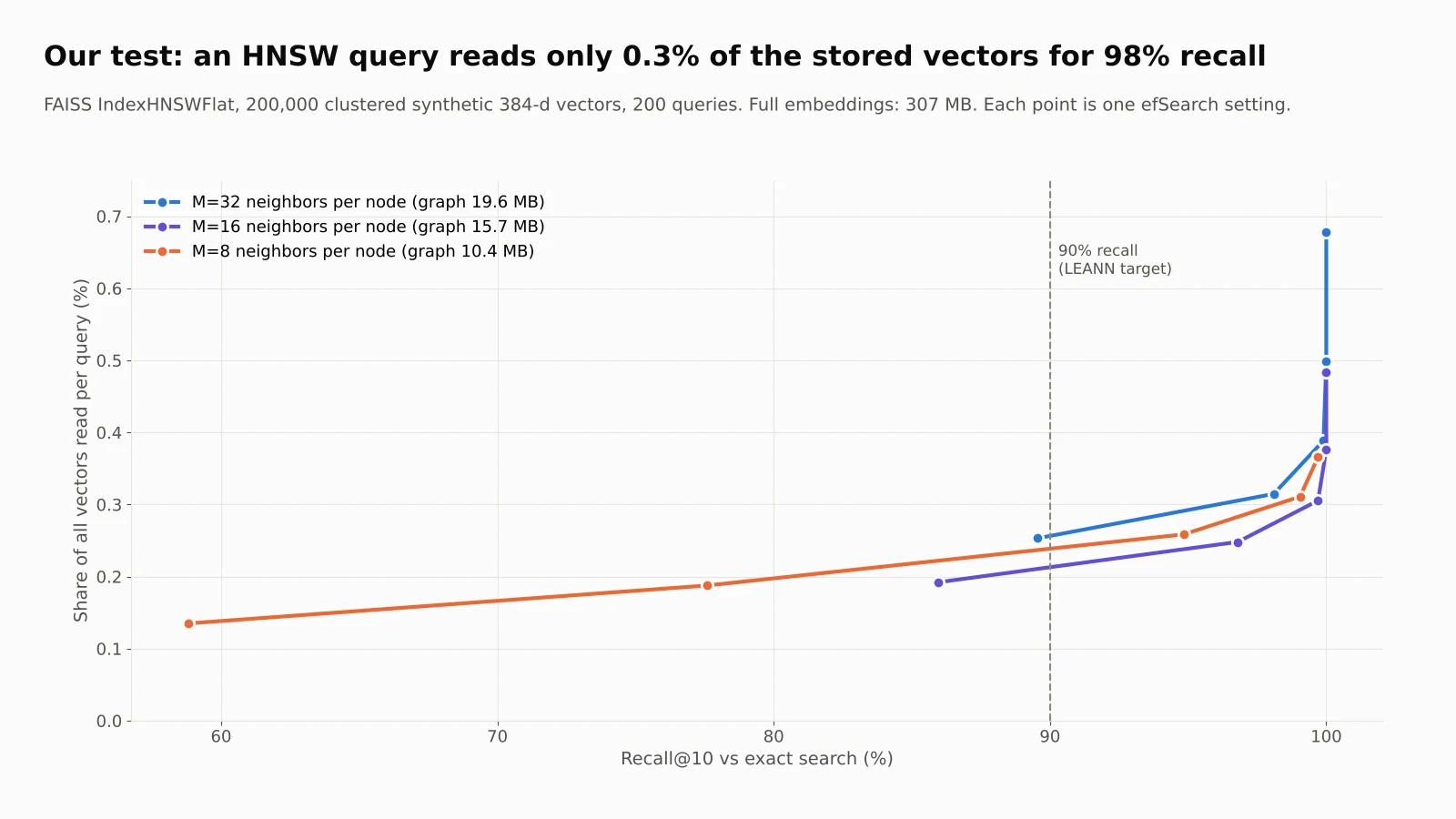
I built FAISS IndexHNSWFlat indexes over 200,000 clustered synthetic 384-dimension vectors (about 307 MB of float32 embeddings) and counted how many distance computations each of 200 queries performed, against exact brute-force search as ground truth. The script is included with this article.
M=32 ef= 16 recall@10=0.896 vectors touched/query=    506 (0.25% of 200,000) graph=19.6 MB
M=32 ef= 32 recall@10=0.981 vectors touched/query=    629 (0.31% of 200,000) graph=19.6 MB
M=32 ef= 64 recall@10=0.999 vectors touched/query=    777 (0.39% of 200,000) graph=19.6 MB
M=16 ef= 32 recall@10=0.968 vectors touched/query=    496 (0.25% of 200,000) graph=15.7 MB
M= 8 ef= 32 recall@10=0.776 vectors touched/query=    375 (0.19% of 200,000) graph=10.4 MB
M= 8 ef= 64 recall@10=0.949 vectors touched/query=    517 (0.26% of 200,000) graph=10.4 MB
Three things stood out:
Each query touched about 0.3% of the vectors. With 32 neighbors per node, 629 vectors out of 200,000 were enough for 98.1% recall. The other 99.7% sat on disk unused for that query.
The graph is small next to the embeddings. The neighbor lists took about 19.6 MB, compared with 307 MB of embeddings, roughly 6%. That's exactly why LEANN keeps the graph and drops the vectors.
Cutting edges naively hurts. Dropping to 8 neighbors per node shrank the graph by about half, but recall at the same search effort fell from 98.1% to 77.6%. That's why LEANN doesn't prune uniformly, as you'll see below.
This was synthetic data, not real text embeddings, and 200,000 vectors rather than 60 million. But it shows the principle clearly. And because the number of nodes an HNSW search visits grows roughly logarithmically with the size of the index, the fraction touched gets even smaller as the dataset grows. The paper makes the same point: the number of recomputed chunks in LEANN grows polylogarithmically with the number of items.
How the LEANN vector index works
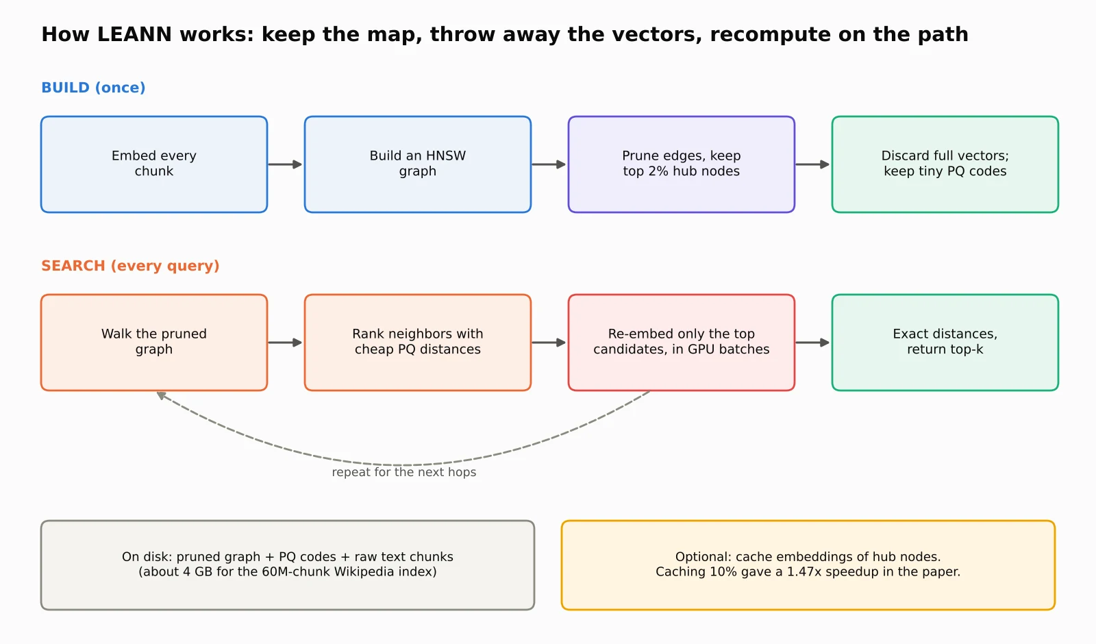
Naive recomputation would be slow, and the graph itself still takes space. LEANN adds three techniques to fix both problems.
1. Two-level search with cheap and exact distances
At each step, LEANN first scores all neighbors using approximate distances from PQ codes, which are tiny and fast. It then picks only the most promising fraction and recomputes their exact embeddings for precise ranking. A global queue of approximate scores lets the search go back to earlier candidates that start to look better later.
In the paper's setup, about 2 GB of PQ codes stand in for roughly 200 GB of full-precision vectors during this first pass. On its own, the two-level search gave an average 1.40x speedup (up to 1.64x) over naive recomputation.
2. Dynamic batching for the GPU
Recomputing a few embeddings at a time wastes a GPU, which is fastest when it processes many inputs at once. LEANN collects candidates across several search hops until it reaches a batch size the hardware likes (for example, 64 on an NVIDIA A10) and embeds them together. This slightly relaxes the strict order of best-first search but keeps the GPU busy. Adding batching raised the total speedup to 1.76x on average, up to 2.02x.
Even with these tricks, embedding recomputation still accounts for about 76% of LEANN's query time, according to the paper's latency breakdown.
3. Pruning that keeps the hubs
Without embeddings, the graph becomes the main storage cost. A typical HNSW node stores dozens of 4-byte neighbor IDs, which can add more than 25% overhead relative to a 256-token text chunk.
LEANN's answer is high-degree preserving graph pruning. The authors observed that searches pass through a small set of highly connected "hub" nodes far more often than others. So LEANN cuts most nodes down to a few edges but lets the top 2% of nodes by degree keep many more. In the paper's ablation, halving the graph's edges this way performed about as well as the unpruned graph, while a "small M" approach (just lowering the neighbor limit, like my M=8 test above) was up to 5.76x worse.
Putting the storage back together
Here's a back-of-envelope reconstruction of where LEANN's roughly 4 GB goes, using numbers from the paper:
Pruned graph:  60M nodes × ~9 avg edges (half of the original 18) × 4 bytes ≈ 2.2 GB
PQ codes:      ~2 GB in the paper's setup (about 32 bytes per vector)
Total:         ≈ 4 GB, about 5% of the 76 GB of raw text
That's my own arithmetic, not a figure from the paper, but it lines up with the reported 4 GB. If you have spare disk, LEANN can also cache the embeddings of hub nodes. Caching just 10% of embeddings gave a 1.47x speedup, with a cache hit rate of up to 41.9%.
What the benchmarks show
All results below are self-reported by the LEANN team, measured at 90% Recall@3 against a 60-million-passage Wikipedia datastore on four standard question-answering benchmarks: NQ, TriviaQA, GPQA and HotpotQA.
| Index | Storage (76 GB corpus) | NQ retrieval at 90% recall | NQ downstream accuracy | Fits a 32 GB RAM workstation |
|---|---|---|---|---|
| LEANN | 4 GB | 2.48 s | 25.5% | Yes |
| HNSW (FAISS) | 188 GB | 0.05 s | 25.5% | No (out of memory) |
| DiskANN | 270 GB | 0.03 s | Not disclosed | Yes |
| IVF recomputation (EdgeRAG-style) | Under 5% of raw data | 307.61 s | Not disclosed | Yes |
| PQ compression | 20 GB | Can't reach 90% recall | 17.9% | Yes |
Figures from the LEANN paper (v2), as summarized by MarkTechPost, using an RTX 4090 and Qwen3-4B for generation. BM25 keyword search scored 18.3% on NQ.
A few takeaways:
Accuracy is preserved. At 90% recall, LEANN's answers were as accurate as HNSW's on NQ, and it improved exact match by up to 11.8% over BM25 keyword search.
It's far faster than the previous recompute approach. The original paper reports LEANN as 21x to 200x faster than an IVF-based recomputation baseline inspired by EdgeRAG.
It's slower than a full index. Retrieval across datasets on the RTX 4090 ranged from 1.12 seconds (GPQA) to 7.12 seconds (HotpotQA). The slowest case was HotpotQA on an M1 Ultra Mac at 44.80 seconds.
HNSW didn't even fit. On the Mac test machine with 128 GB of RAM, HNSW and IVF ran out of memory because the embeddings alone exceeded the RAM.
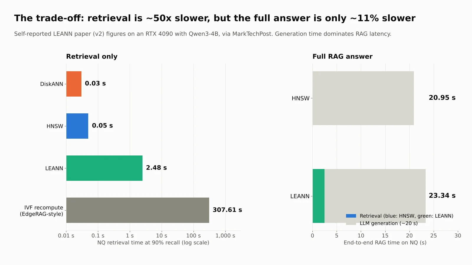
That last chart is the most important framing in the whole paper. Retrieval time looks terrible in isolation: 2.48 seconds versus 0.05. But in a real RAG pipeline, generating the answer with a local LLM took about 20 seconds. End to end, the answer arrived in 23.34 seconds with LEANN versus 20.95 seconds with HNSW. For a personal assistant on your laptop, that's a reasonable price for using 4 GB of disk instead of 188 GB.
How to install and try LEANN
The package is MIT licensed and published on PyPI. The default install includes the HNSW, DiskANN and IVF backends:
uv pip install leann
The basic Python API, from the project's README, has three parts: build an index, search it and chat with it.
from leann import LeannBuilder, LeannSearcher, LeannChat
from pathlib import Path

INDEX_PATH = str(Path("./").resolve() / "demo.leann")

# Build an index
builder = LeannBuilder(backend_name="hnsw")  # or "diskann" / "ivf"
builder.add_text("LEANN saves 97% storage compared to traditional vector databases.")
builder.add_text("Tung Tung Tung Sahur called—they need their banana-crocodile hybrid back")
builder.build_index(INDEX_PATH)

# Search
searcher = LeannSearcher(INDEX_PATH)
results = searcher.search("fantastical AI-generated creatures", top_k=1)

# Chat with your data
chat = LeannChat(INDEX_PATH, llm_config={"type": "hf", "model": "Qwen/Qwen3-0.6B"})
response = chat.ask("How much storage does LEANN save?", top_k=1)
The first run downloads an embedding model, and recomputation is much faster with a GPU or Apple Silicon. The README also documents a CPU-only install for Linux, though the team hasn't published CPU latency numbers. MarkTechPost reports support for Ubuntu, Arch, WSL, macOS and Windows, with some apps such as Apple Mail search limited to macOS. For generation, LEANN works with Ollama, Hugging Face, Anthropic or any OpenAI-compatible API.
A practical tip from the ecatech write-up that I agree with: start with a small personal dataset, such as your browser history or a folder of documents, to see how search latency feels on your hardware before you index anything large.
What you can build with it
According to the project, LEANN ships with ready-made apps for:
Local documents: semantic search and chat over your own files.
Personal data: Apple Mail, Chrome browser history, WeChat, iMessage and exported ChatGPT or Claude conversations.
Live sources through MCP: readers that pull data from Slack and Twitter bookmarks.
Code search for AI agents: LEANN can run as a semantic search MCP server for Claude Code.
The repo's personal-data numbers show where the savings matter most: 400,000 chat messages shrink from 1.8 GB to 64 MB, and 38,000 browser history entries shrink from 130 MB to 6.4 MB.
The code search result is interesting for agent builders. On 30 SWE-Bench Pro tasks from ContextBench, the team reports that LEANN found relevant code with 24.2% initial recall versus 11.4% for BM25, and the agent used 8.4% fewer tokens. If you're building coding agents, our guide to how agentic AI works explains why better retrieval tools make such a difference to agent cost and quality.
When to use the LEANN vector index, and when not to
| Situation | Best choice | Why |
|---|---|---|
| Personal or on-device RAG on a laptop | LEANN | Storage is the bottleneck, and a few seconds of search is acceptable |
| Private data that must stay local | LEANN | Small enough to index mail, chats and files without a server |
| Production search with many users and millisecond SLAs | HNSW or DiskANN | You need sub-100 ms retrieval and can afford the storage |
| Billion-scale search on servers with fast SSDs | DiskANN | Built for large disk-resident indexes with very low latency |
| Keyword-heavy queries (IDs, exact phrases) | BM25 or hybrid search | Embeddings aren't the right tool for exact matching |
LEANN is a specialist. It's at its best when disk space is scarce and a person is waiting for an answer that an LLM will take many seconds to write anyway.
Limitations to know before you adopt it
Search takes seconds, not milliseconds. That's fine for a personal assistant and wrong for a high-traffic API.
Building the index still needs the full embeddings. The paper says LEANN must compute embeddings for all passages before building the graph, so peak storage during construction can be high. The authors suggest building cluster by cluster as one workaround.
You need the embedding model at query time. Because LEANN recomputes embeddings, every search runs the embedding model. That uses compute and, on a laptop, battery. You'll also want to pin the exact model version, since changing it means rebuilding the index.
The numbers are self-reported. All benchmarks come from the LEANN team. They're detailed and consistent with the method, but they haven't yet been independently reproduced at full scale.
Model size is a lever. Recomputation dominates latency, so a smaller embedder helps. In the paper, swapping the 110M-parameter Contriever for the 34M-parameter GTE-small gave a 2.3x speedup on a 2M-chunk datastore while keeping downstream accuracy within 2%.
My take
LEANN is one of those ideas that feels obvious once someone has done it. If a query only reads 0.3% of your index, storing 100% of the expensive part is wasteful. The clever work is in making recomputation fast enough to be useful: the two-level search, the batching and especially the hub-preserving pruning.
What I like most is how honestly the trade-off fits the use case. Nobody needs 50 ms retrieval for a personal assistant that takes 20 seconds to write its answer. People do need their laptop's disk. LEANN trades a resource that's plentiful in that setting (a few seconds of compute) for one that's scarce (hundreds of gigabytes of storage).
I'd treat it as the strongest current option for local, private RAG, and keep using HNSW or DiskANN for production services with strict latency targets. I'd also watch it closely as consumer GPUs and small embedding models get faster, because every improvement there shrinks LEANN's one real weakness. If inference cost is your concern more broadly, ByteMuni's look at DeepSeek's DeepInfer tool covers the other side of the same problem.
The bottom line
The LEANN vector index makes semantic search over large collections practical on ordinary hardware. By storing a pruned graph and compact PQ codes, then recomputing exact embeddings only along each search path, it cuts a 60-million-chunk Wikipedia index from 201 GB to 6 GB (or 188 GB to 4 GB in the paper's comparison) while matching HNSW's answer quality at 90% recall. The cost is a few seconds per search, which matters far less once an LLM is writing the answer.
If you want private RAG over your own documents, mail or code on a laptop, it's well worth a try: uv pip install leann, start small and measure. More AI tooling coverage is in ByteMuni's AI & Machine Learning section.
Sources
LEANN: A Low-Storage Vector Index — Wang et al., UC Berkeley, arXiv 2506.08276
Meet LEANN: an open-source vector index that shrinks a 60M-chunk RAG index from 201 GB to 6 GB — MarkTechPost, Oct 27, 2026
Meet LEANN — ecatech, Oct 28, 2026
LEANN on PyPI — package and README (version 0.3.8, MIT license)
LEANN on GitHub — source code
Frequently asked questions
What is LEANN?
LEANN is an open-source, MIT-licensed vector index from UC Berkeley's Sky Computing Lab. It is designed for low storage: instead of saving every embedding, it keeps a pruned search graph and compact PQ codes, and recomputes exact embeddings only for the chunks a query visits.
How does LEANN reduce vector index size?
It drops full-precision embeddings, which are usually the biggest part of an index, prunes the graph while keeping the top 2% of highly connected hub nodes, and stores small product quantization codes for fast approximate scoring. In the paper, this brings storage to under 5% of the raw data.
Is LEANN as accurate as HNSW?
According to the LEANN team, yes at the same recall target. At 90% recall, LEANN and HNSW both reached 25.5% downstream accuracy on NQ. Pure PQ compression at a similar size scored 17.9% and couldn't reach 90% recall.
How fast is LEANN?
Slower than a full in-memory index. On an RTX 4090, LEANN's NQ retrieval took 2.48 seconds versus 0.05 seconds for HNSW, and HotpotQA took 7.12 seconds. Because LLM generation took about 20 seconds, end-to-end RAG time rose only from 20.95 to 23.34 seconds.
How do I install LEANN?
Run uv pip install leann (or pip install leann). The default install includes HNSW, DiskANN and IVF backends. The Python API uses LeannBuilder to build an index, LeannSearcher to search and LeannChat to ask questions with an LLM.
When should I not use LEANN?
Avoid it for high-traffic production search that needs millisecond latency, where HNSW or DiskANN fit better, and for exact keyword lookups, where BM25 or hybrid search works better. Also note that building the index still needs all embeddings temporarily.
How we research, write and check articles