How to Train a Neural Network in PyTorch Without Data Leakage

To train a neural network in PyTorch without data leakage, split your data before you touch it, fit every scaler on the training rows only, pick epochs and settings with a validation set, and look at the test set exactly once. I ran that workflow on the classic 10-row salary dataset, then repeated it 50 times to see what actually moves the score.

The short version of what I found: the order of operations matters, but on a dataset this small, which rows land in your test set matters even more. One random split gave a test error of $1.8k. Another, with identical code, gave $199k.

Below is the full, runnable code, the numbers from my runs, and the three bugs I keep finding in copy-paste tutorials on this exact example.

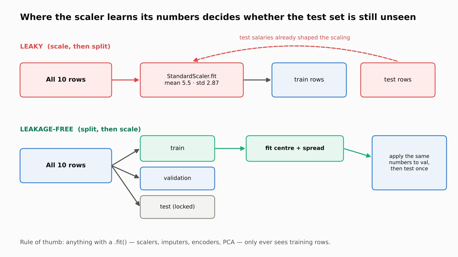
Fit the scaler before the split and the test salaries have already shaped your preprocessing. Split first and the test rows stay genuinely unseen.

What data leakage looks like in a 10-row dataset

Data leakage is any path by which information from your evaluation rows reaches the model before evaluation. The usual culprit isn't the model. It's preprocessing.

Here's the version you'll see in a lot of beginner tutorials, including ProjectPro's salary example:

# Leaky: the scaler sees every row, including future test rows
x_scaled = scaler_x.fit_transform(x)
y_scaled = scaler_y.fit_transform(y)
x_train, x_test, y_train, y_test = train_test_split(x_scaled, y_scaled, test_size=0.2)

fit_transform on the full dataset computes the mean and standard deviation from all 10 rows. On this data that's a salary mean of $249,500 and a standard deviation of about $284,000, and both numbers are heavily pulled by the CEO's $1,000,000. If the CEO row later ends up in the test set, your training data was scaled using a number that only exists because of a test row.

scikit-learn's own documentation on common pitfalls puts it plainly: call fit only on training data, then transform everything else with what you learned. That applies to anything with a .fit() method: scalers, imputers, encoders, PCA, feature selectors.

Set up the project

You need four libraries to train a neural network in PyTorch for this example. No pre-trained model, no GPU.

pip install pandas torch scikit-learn matplotlib

I tested everything below on Python 3.13, PyTorch 2.14 (CPU build) and scikit-learn 1.9. Older versions from the last couple of years should work; nothing here uses new APIs.

Save this as Position_Salaries.csv. It's the widely used 10-row dataset from the Kaggle "Position Salaries" example, so you don't need to go hunting for a download link:

Position,Level,Salary
Business Analyst,1,45000
Junior Consultant,2,50000
Senior Consultant,3,60000
Manager,4,80000
Country Manager,5,110000
Region Manager,6,150000
Partner,7,200000
Senior Partner,8,300000
C-level,9,500000
CEO,10,1000000

Notice the shape before writing any code: salary roughly doubles every couple of levels, then jumps 2x from C-level to CEO. That's exponential growth, and it will matter when we pick a target.

Load the data and fail loudly

import numpy as np
import pandas as pd
import torch
from torch import nn
from sklearn.model_selection import train_test_split
from sklearn.preprocessing import StandardScaler

torch.manual_seed(42)

df = pd.read_csv("Position_Salaries.csv")
assert df[["Level", "Salary"]].notna().all().all(), "Fix missing values before training"

X = df[["Level"]].to_numpy(dtype=np.float32)    # shape (10, 1)
y = df[["Salary"]].to_numpy(dtype=np.float32)   # shape (10, 1)

Two small choices here are deliberate.

I select columns by name instead of data.values[:, 1]. Positional indexing works until someone adds an ID column to the CSV, and then your model silently trains on the wrong feature.

I also skip df.apply(pd.to_numeric, errors="coerce"). Many tutorials use it to "handle non-numeric data", but it doesn't handle anything. It turns bad values into NaN and carries on. A NaN in a PyTorch tensor turns your loss into nan a few lines later, far from the real cause. An assert at load time is cheaper to debug.

Split first: train, validation and test

X_dev, X_test, y_dev, y_test = train_test_split(X, y, test_size=0.2, random_state=7)
X_train, X_val, y_train, y_val = train_test_split(X_dev, y_dev, test_size=0.25, random_state=7)
print(f"train={len(X_train)} val={len(X_val)} test={len(X_test)}")
# train=6 val=2 test=2

Three sets, three jobs:

• Training rows update the weights.

• Validation rows help you choose: how many epochs, how many layers, which learning rate.

• Test rows answer one question at the very end: how wrong is this model on data it has never influenced?

The moment you change something because of the test score, the test set has become a second validation set and you no longer have an honest estimate. ProjectPro's training loop prints test loss every 10 epochs, which invites exactly that kind of peeking.

Be honest about the numbers here, though: 6 training rows, 2 validation rows, 2 test rows. That's thin. I'll come back to what that does to your results, because it's the most interesting part of this experiment.

Fit the scalers on training rows only

x_scaler = StandardScaler().fit(X_train)
y_scaler = StandardScaler().fit(np.log(y_train))

def to_tensor(a):
    return torch.tensor(a, dtype=torch.float32)

Xtr = to_tensor(x_scaler.transform(X_train))
ytr = to_tensor(y_scaler.transform(np.log(y_train)))
Xva = to_tensor(x_scaler.transform(X_val))
yva = to_tensor(y_scaler.transform(np.log(y_val)))

fit happens once, on X_train and y_train. Validation (and later, test) data only gets transform.

You'll notice I scale np.log(y_train) rather than raw salary. Because salaries grow roughly exponentially with level, the log of salary is close to a straight line. That's an easier shape for a small network to learn from six points, and it keeps the CEO's million from dominating the squared-error loss. In my cross-validation runs this one change cut the error by about 40%. Numbers below.

Train a neural network in PyTorch with early stopping

The architecture is the same small regression network most tutorials use for this dataset: one input, two hidden layers of 64 ReLU units, one output.

def make_model():
    return nn.Sequential(
        nn.Linear(1, 64), nn.ReLU(),
        nn.Linear(64, 64), nn.ReLU(),
        nn.Linear(64, 1),
    )

model = make_model()
loss_fn = nn.MSELoss()
optimizer = torch.optim.Adam(model.parameters(), lr=0.01)

best_val, best_state, patience, bad_epochs = float("inf"), None, 30, 0
for epoch in range(500):
    model.train()
    loss = loss_fn(model(Xtr), ytr)
    optimizer.zero_grad()
    loss.backward()
    optimizer.step()

    model.eval()
    with torch.inference_mode():
        val_loss = loss_fn(model(Xva), yva).item()

    if val_loss < best_val - 1e-6:
        best_val, bad_epochs = val_loss, 0
        best_state = {k: v.clone() for k, v in model.state_dict().items()}
    else:
        bad_epochs += 1
        if bad_epochs >= patience:
            print(f"stopped at epoch {epoch}, best val loss {best_val:.5f}")
            break

model.load_state_dict(best_state)

A few notes from a developer's point of view:

• The whole training set is one batch. With six rows, mini-batches add nothing. On real data, wrap your tensors in a DataLoader and loop over batches.

• Validation decides when to stop. Instead of hard-coding 100 epochs, the loop keeps the weights from the best validation epoch and stops after 30 epochs without improvement. On my run it stopped at epoch 57.

• .clone() matters. state_dict() returns references to live tensors. Without cloning, your "best" checkpoint quietly keeps updating with the model and you restore the final weights, not the best ones. PyTorch's saving and loading guide covers this in more detail.

• model.eval() and torch.inference_mode() don't change anything for this particular network, which has no dropout or batch norm. Keep them anyway. The day you add dropout, forgetting eval() makes validation scores noisy in a way that's hard to spot.

Score the test set once, in salary units

def predict_salary(model, levels):
    model.eval()
    with torch.inference_mode():
        scaled = model(to_tensor(x_scaler.transform(levels))).numpy()
    return np.exp(y_scaler.inverse_transform(scaled))

test_pred = predict_salary(model, X_test)
mae = np.abs(test_pred - y_test).mean()
print(f"Held-out MAE: ${mae:,.0f}")
# Held-out MAE: $16,173  (test levels 9 and 6)

Every prediction goes through the same three steps: scale the input with the training scaler, run the network, then undo the target transform (inverse scaling, then exp). Wrapping that in one predict_salary function means the plot, the test score and any future API endpoint can't drift apart.

Report the error in salary units, not scaled units. "MSE 0.00002" means nothing to the person who asked for the model. "Off by about $16k on average" does.

What happened when I ran it 50 times

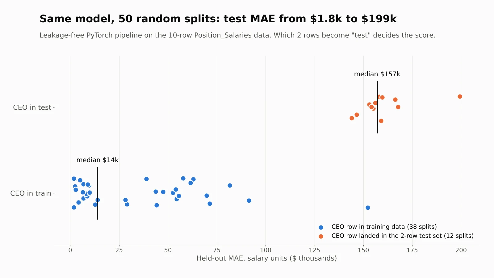
A single test score of $16,173 looked good. So I reran the whole leakage-free pipeline with 50 different random splits, same code, same model, same 80/20 ratio.

Same model, same code, 50 splits. When the $1M CEO row lands in the two-row test set, the median error jumps from about $14k to $157k.

The test MAE ranged from $1,752 to $199,369. The median was $45,799.

The split explains almost all of it. In 12 of the 50 splits, the CEO row ended up in the test set. Those runs had a median error of $157,047. In the other 38, the median was $13,947. The network never saw a salary above $500k, and ReLU networks extrapolate in straight lines, so it had no way to guess the jump to a million.

Then I compared against the leaky pipeline (scale everything, then split) on the same 50 splits. I expected the leak to make the scores look better. It didn't: the leaky version had a slightly worse median ($50,750) and beat the clean version in only 16 of 50 splits.

That's worth being straight about. Leakage doesn't always inflate a score, especially when the leaked information is just one mean and one standard deviation. The point of splitting first isn't that it raises or lowers your number. It's that the clean number means what it says. With target encoders, imputers or feature selection fitted on the full data, the leak carries far more information about the test rows, and the optimistic bias gets much bigger. scikit-learn's pitfalls page walks through a feature-selection example of exactly that.

The bigger lesson from this chart: a single random split on a tiny dataset is close to a coin flip. Don't report one.

Use leave-one-out cross-validation when data is this small

If you train a neural network in PyTorch on 10 rows, the better evaluation is leave-one-out cross-validation (LOOCV): train on 9 rows, predict the 10th, repeat for every row, average the errors. Every row gets to be the test row exactly once, and the scalers are refit inside every fold.

from sklearn.model_selection import LeaveOneOut

def loocv_mae(X, y, epochs=100, seeds=(0, 1, 2)):
    errors = []
    for train_idx, test_idx in LeaveOneOut().split(X):
        xs = StandardScaler().fit(X[train_idx])            # refit per fold
        ys = StandardScaler().fit(np.log(y[train_idx]))
        Xt = to_tensor(xs.transform(X[train_idx]))
        yt = to_tensor(ys.transform(np.log(y[train_idx])))
        preds = []
        for seed in seeds:                                  # average out init noise
            torch.manual_seed(seed)
            m = make_model()
            opt = torch.optim.Adam(m.parameters(), lr=0.01)
            for _ in range(epochs):
                m.train()
                l = loss_fn(m(Xt), yt)
                opt.zero_grad(); l.backward(); opt.step()
            m.eval()
            with torch.inference_mode():
                p = m(to_tensor(xs.transform(X[test_idx]))).numpy()
            preds.append(np.exp(ys.inverse_transform(p))[0, 0])
        errors.append(abs(np.mean(preds) - y[test_idx][0, 0]))
    return float(np.mean(errors)), errors

mean_err, per_row = loocv_mae(X, y)
print(f"LOOCV MAE: ${mean_err:,.0f}")
# LOOCV MAE: $29,305  (worst row: the CEO, off by $204k)

There's no validation split inside each fold, so this uses a fixed 100 epochs rather than early stopping. Treat the epoch count as a setting you chose once up front, not something you tune against the LOOCV score.

I used the same LOOCV setup (5 seeds per fold this time) to compare four approaches:

ApproachLOOCV MAEMAE excluding CEO rowPredicted CEO salaryLinear regression on salary$170,556$123,890$409,444Linear regression on log(salary)$67,808$24,442$541,891PyTorch net on scaled salary$45,919$17,674$699,874PyTorch net on log(salary)$27,940$9,352$804,767

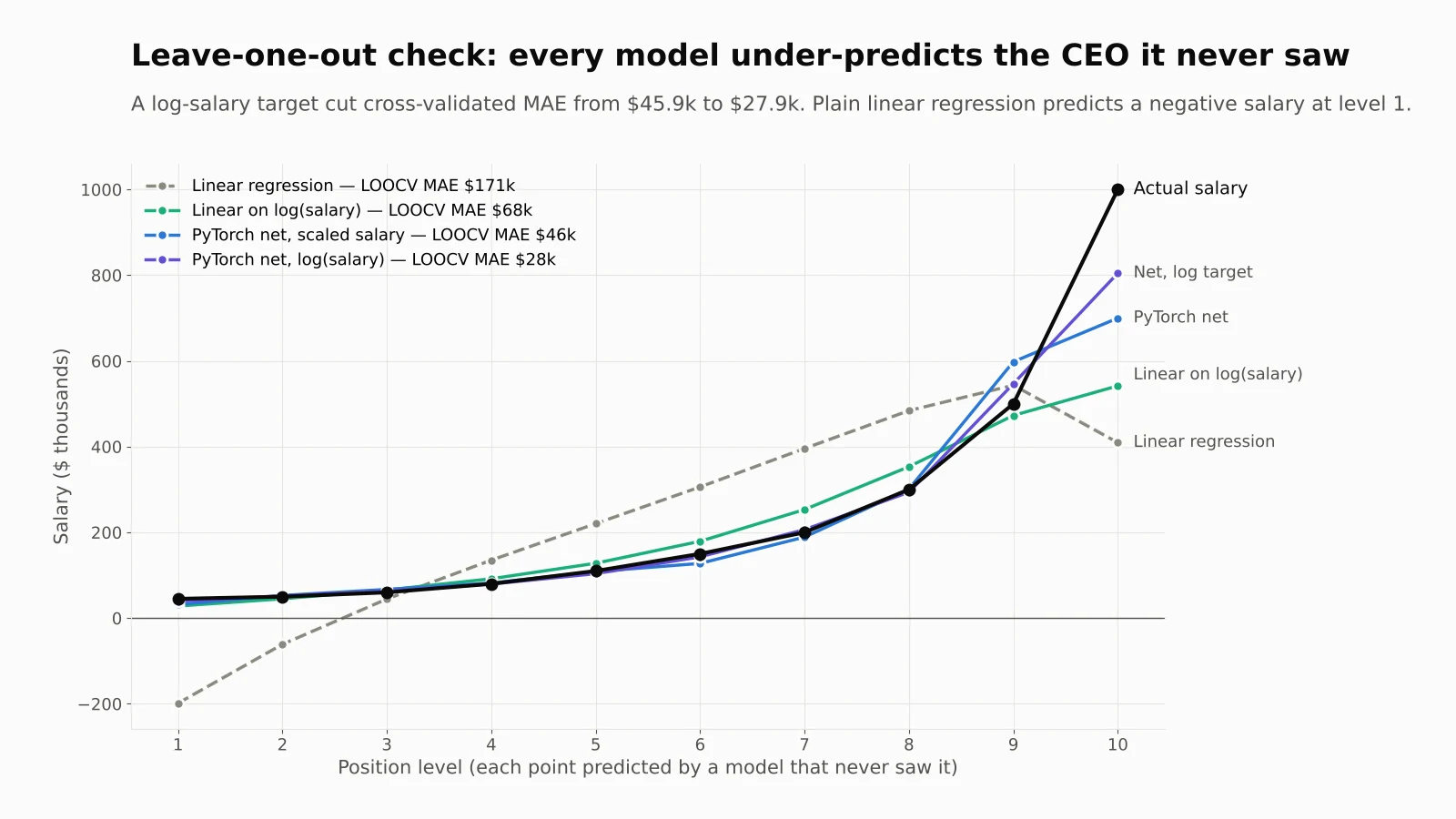
Each point is predicted by a model that never saw that row. The log-target network tracks the curve best, and every approach still under-predicts the CEO.

Three takeaways from that table:

1. The neural network earned its place here. Plain linear regression predicts a negative salary (−$198,611) for level 1 when that row is held out. The relationship is curved, and the network's ReLU layers can bend.

2. The target transform mattered as much as the model. Switching the network to log(salary) cut LOOCV error by about 40%. Before you add layers, look at the shape of your target.

3. Nothing extrapolates to the CEO. The best model still predicts about $805k for a $1M row. If your real data has outliers at the edge of the range, no amount of tuning on interior points will fix that. You need more data near the edge or a model with the right shape built in.

Three bugs to check in tutorials you copy

I went through the two most-shared versions of this tutorial line by line. These are the issues worth fixing before you reuse their code.

1. Scaling before splitting (ProjectPro). Covered above. Move fit after train_test_split.

2. Plotting raw inputs through a model trained on scaled inputs (ProjectPro). The final plot calls model(x) on unscaled levels 1 to 10, while the network was trained on standardized inputs between roughly −1.6 and +1.6. The resulting curve is meaningless, and it's easy to blame the architecture for it. Route plots through the same predict_salary function you use for scoring:

import matplotlib.pyplot as plt

plt.plot(X, y, "o-", label="Actual")
plt.plot(X, predict_salary(model, X), "o--", label="Model")
plt.xlabel("Position level"); plt.ylabel("Salary"); plt.legend(); plt.show()

This plot includes training rows, so use it to sanity-check the curve, not as evidence of accuracy.

ProjectPro's Step 7 also defines the loss and optimizer twice (first L1Loss with SGD for 1,000 epochs, then MSELoss with Adam for 100). Only the second block takes effect. Delete the first so nobody wonders which one ran.

3. Outdated Hugging Face arguments (dev.to fine-tuning guide). If you move from this numeric example to fine-tuning a text model like DistilBERT, watch two things in older guides. TrainingArguments(evaluation_strategy=...) was renamed to eval_strategy; recent transformers releases reject the old name with a TypeError. And transformers.convert_graph_to_onnx is deprecated; export with Hugging Face Optimum instead (optimum-cli export onnx). The same guide also passes the test split as eval_dataset and evaluates every epoch, which is the same test-set peeking problem in a different framework. Carve a validation split out of the training data and keep the test split for the end.

When a neural network is the wrong tool

This example is good for learning the mechanics. It isn't a template for a real compensation model, and I'd push back if someone tried to ship it as one.

• One feature isn't a salary model. Position level alone ignores location, experience, company size and everything else that drives pay. Predicting recorded salary also bakes in whatever past pay decisions produced those records, including any bias in them.

• Try the simple baseline first. Here a log-linear regression reached $24k LOOCV error on the non-CEO rows with zero training loop. On many tabular problems a linear model or a gradient-boosted tree beats a neural network and is easier to explain. Use the network when the baseline clearly loses, as it did here on the full range.

• Random splits aren't always valid. If rows have timestamps, split chronologically so the model never trains on the future. If the same person or entity appears multiple times, use a group-aware split such as scikit-learn's GroupKFold so duplicates can't sit on both sides of the boundary.

Before this goes anywhere near production

A clean training loop is the start, not the finish. At minimum:

• Save the preprocessing with the model. The x_scaler and y_scaler objects are part of the model. Persist them (for example with joblib) alongside the PyTorch state_dict, and load both together. Mismatched scalers are one of the most common silent bugs in deployed models.

• Version the data, not just the code. Record which CSV, which split seed and which library versions produced each model.

• Monitor inputs, not only errors. Log when a request arrives with a level outside the training range. That's exactly where this model is weakest.

• Retrain with the same pipeline. Fit scalers on new training data every time, then re-run the same validation and a fresh, untouched test check.

Whenever you train a neural network in PyTorch, or in any other framework, here's the order to remember: split → fit preprocessing on train → tune on validation → test once → report in real units. Everything else in this post is detail around those five steps.

Sources

• How to Build an AI Model from Scratch? — ProjectPro (original salary example)

• Building Your Own AI Model with Open-Source Tools — dev.to

• Common pitfalls and recommended practices — scikit-learn documentation

• Saving and loading models — PyTorch tutorials

• Export a model to ONNX with Optimum — Hugging Face documentation